physicsgen
PhysicsGen: Can Generative Models Learn from Images
to Predict Complex Physical Relations?
AbstractThe image-to-image translation abilities of generative learning models have recently made significant progress in the estimation of complex (steered) mappings between image distributions. While appearance based tasks like image in-painting or style transfer have been studied at length, we propose to investigate the potential of generative models in the context of physical simulations. Providing a dataset of 300k image-pairs and baseline evaluations for three different physical simulation tasks, we propose a benchmark to investigate the following research questions: i) are generative models able to learn complex physical relations from input-output image pairs? ii) what speedups can be achieved by replacing differential equation based simulations? While baseline evaluations of different current models show the potential for high speedups (ii), these results also show strong limitations toward the physical correctness (i). This underlines the need for new methods to enforce physical correctness. |
|
Download Datasets & Hugging Face Datasets
The dataset used for evaluation, which contains 300k image pairs across three diverse simulation scenarios, is publicly available via Zenodo ![]() and also available through Hugging Face Datasets.
and also available through Hugging Face Datasets.
Variants
-
Urban Sound Propagation: [sound_baseline, sound_reflection, sound_diffraction, sound_combined]
Each sound example includes:
- Geographic coordinates:
lat,long - Sound intensity:
db - Images:
soundmap,osm,soundmap_512 - Additional metadata:
temperature,humidity,yaw,sample_id
- Geographic coordinates:
-
Lens Distortion: [lens_p1, lens_p2]
Each lens example includes:
- Calibration parameters:
fx,k1,k2,k3,p1,p2,cx - Label file path:
label_path - Note: The script for applying the distortion to the CelebA Dataset is located here.
- Calibration parameters:
-
Dynamics of rolling and bouncing movements: [ball_roll, ball_bounce]
Each ball example includes:
- Metadata:
ImgName,StartHeight,GroundIncli,InputTime,TargetTime - Images:
input_image,target_image
- Metadata:
Data is divided into train, test, and eval splits. For efficient storage and faster uploads, the data is converted and stored as Parquet files with image data stored as binary blobs.
Usage
You can load and use the dataset with the Hugging Face datasets library. For example, to load the sound_combined variant:
from datasets import load_dataset

dataset = load_dataset("mspitzna/physicsgen", name="sound_combined", trust_remote_code=True)

# Access a sample from the training split.
sample = dataset["train"][0]
input_img = sample["osm"]
target_img = sample["soundmap_512"]

# plot Input vs Target Image for a single sample
fig, (ax1, ax2) = plt.subplots(1, 2, figsize=(10, 5))
ax1.imshow(input_img)
ax2.imshow(target_img)
plt.show()
Code for baseline experiments
The code is located in the GitHub repository.
Project Structure:
project_root/
│
├── data/                         # Dedicated data folder
│   └── urban_sound_25k_baseline/ # Download this via provided DOI
│       ├── test/
│       │   ├── test.csv
│       │   ├── soundmaps/
│       │   └── buildings/
│       │
│       └── pred/                 # Your predictions
│           ├── y_0.png
│           └── ...
│
└── eval_scripts/
    ├── lens_metrics.py
    └── sound_metrics.py
The indexing system for predicted sound propagation images in the pred folder aligns directly with the test.csv dataframe rows. Each predicted image file, named as y_{index}.png, corresponds to the test data’s row at the same index, with index 0 referring to the dataframe’s first row.
Sound Propagation Evaluation Script
Description: Evaluates sound propagation predictions by comparing them to ground truth noise maps, including Line-of-Sight (LoS) and Non-Line-of-Sight (NLoS) errors.
Usage:
python sound_metrics.py --data_dir data/true --pred_dir data/pred --output evaluation.csv
Arguments:
--data_dir: Directory containing true sound maps andtest.csv.--pred_dir: Directory containing predicted sound maps.--output: Path to save the evaluation results.
Lens Evaluation Script
Description: Evaluates the accuracy of facial landmark predictions by comparing them to ground truth images.
Usage:
python lens_metrics.py --data_dir data/true --pred_dir data/pred --output results/
Arguments:
--data_dir: Directory containing true label images andtest.csv.--pred_dir: Directory containing predicted landmark images.--output: Directory to save the results.
Results
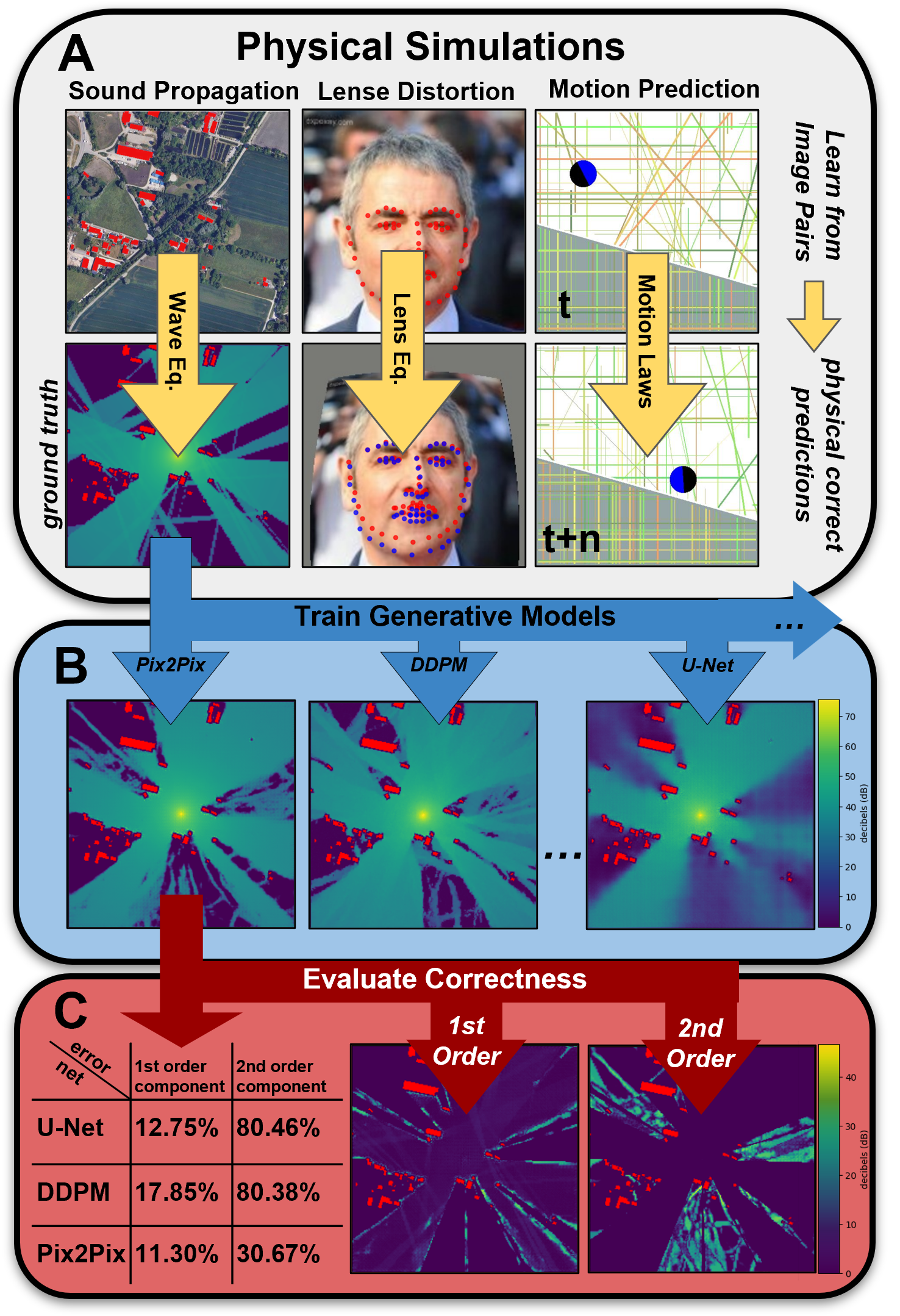
Urban Sound Propagation
The table below presents baseline performance metrics for various architectural approaches, encompassing combined mean absolute error (MAE) and weighted mean absolute percentage error (wMAPE), alongside specific line-of-sight (LoS) and non-line-of-sight (NLoS) metrics.
| Condition | Architecture | LoS MAE | NLoS MAE | LoS wMAPE | NLoS wMAPE | Runtime / Sample (ms) |
|---|---|---|---|---|---|---|
| Baseline | Simulation | 0.00 | 0.00 | 0.00 | 0.00 | 204700 |
| Baseline | convAE | 3.67 | 2.74 | 20.24 | 67.13 | 0.128 |
| Baseline | VAE | 3.92 | 2.84 | 21.33 | 75.58 | 0.124 |
| Baseline | UNet | 2.29 | 1.73 | 12.91 | 37.57 | 0.138 |
| Baseline | Pix2Pix | 1.73 | 1.19 | 9.36 | 6.75 | 0.138 |
| Baseline | DDPM | 2.42 | 3.26 | 15.57 | 51.08 | 3986.353 |
| Baseline | SD(w.CA) | 3.76 | 3.34 | 17.42 | 35.18 | 2961.027 |
| Baseline | SD | 2.12 | 1.08 | 13.23 | 32.46 | 2970.86 |
| Baseline | DDBM | 1.61 | 2.17 | 17.50 | 65.24 | 3732.21 |
| Baseline | Full Glow1 | 1.84 | 0.65 | 8.83 | 4.52 | 101.7 |
| Diffraction | Simulation | 0.00 | 0.00 | 0.00 | 0.00 | 206000 |
| Diffraction | convAE | 3.59 | 8.04 | 13.77 | 32.09 | 0.128 |
| Diffraction | VAE | 3.92 | 8.22 | 14.46 | 32.57 | 0.124 |
| Diffraction | UNet | 0.94 | 3.27 | 4.22 | 22.36 | 0.138 |
| Diffraction | Pix2Pix | 0.91 | 3.36 | 3.51 | 18.06 | 0.138 |
| Diffraction | DDPM | 1.59 | 3.27 | 8.25 | 20.30 | 3986.353 |
| Diffraction | SD(w.CA) | 2.46 | 7.72 | 10.14 | 31.23 | 2961.027 |
| Diffraction | SD | 1.33 | 5.07 | 8.15 | 24.45 | 2970.86 |
| Diffraction | Full Glow1 | 0.79 | 2.63 | 2.43 | 11.12 | 107.62 |
| Reflection | Simulation | 0.00 | 0.00 | 0.00 | 0.00 | 251000 |
| Reflection | convAE | 3.83 | 6.56 | 20.67 | 93.54 | 0.128 |
| Reflection | VAE | 4.15 | 6.32 | 21.57 | 92.47 | 0.124 |
| Reflection | UNet | 2.29 | 5.72 | 12.75 | 80.46 | 0.138 |
| Reflection | Pix2Pix | 2.14 | 4.79 | 11.30 | 30.67 | 0.138 |
| Reflection | DDPM | 2.74 | 7.93 | 17.85 | 80.38 | 3986.353 |
| Reflection | SD(w.CA) | 3.81 | 6.82 | 19.78 | 81.61 | 2961.027 |
| Reflection | SD | 2.53 | 5.26 | 15.04 | 55.27 | 2970.86 |
| Reflection | DDBM | 1.93 | 6.38 | 18.34 | 79.13 | 3732.21 |
| Reflection | Full Glow1 | 2.06 | 3.64 | 8.98 | 22.69 | 102.3 |
Lens Distortion
The table presents a comparative analysis of different models’ performance in accurately predicting facial landmarks under varying lens distortion settings, represented by the coefficients ( p_1 ) and ( p_2 ). It details the combined error, X Error, Y Error, and Shift for each model, highlighting how each model copes with horizontal and vertical distortion impacts separately.
| Model | Comb. | X Err. | Y Err. | Shift | Runtime / Sample (ms) |
|---|---|---|---|---|---|
| $p_1 \neq 0, p_2 = 0$ | |||||
| Simulation | 0.00 | 0.00 | 0.00 | 0.00 | 153.205 |
| convAE | 11.93 | 6.75 | 8.13 | 1.38 | 0.110 |
| VAE | 11.53 | 6.55 | 7.83 | 1.28 | 0.122 |
| UNet | 2.82 | 1.28 | 2.15 | 0.87 | 0.118 |
| Pix2Pix | 2.00 | 0.99 | 1.43 | 0.44 | 0.122 |
| DDPM | 1.93 | 0.94 | 1.39 | 0.45 | 3970.603 |
| SD(w.CA) | 3.09 | 1.59 | 2.21 | 0.62 | 2991.678 |
| SD | 2.79 | 1.41 | 2.01 | 0.60 | 2997.576 |
| $p_1 = 0, p_2 \neq 0$ | |||||
| Simulation | 0.00 | 0.00 | 0.00 | 0.00 | 153.205 |
| convAE | 10.56 | 8.35 | 4.77 | 2.21 | 0.110 |
| VAE | 10.40 | 8.26 | 4.62 | 3.64 | 0.122 |
| UNet | 2.36 | 1.33 | 1.60 | 0.27 | 0.117 |
| Pix2Pix | 1.77 | 1.02 | 1.14 | 0.13 | 0.123 |
| DDPM | 2.13 | 1.39 | 1.23 | 0.16 | 3970.603 |
| SD(w.CA) | 2.85 | 1.60 | 1.94 | 0.34 | 2991.678 |
| SD | 2.44 | 1.38 | 1.64 | 0.26 | 2997.576 |
Dynamics of rolling and bouncing movements
The table evaluates the performance of three generative models—GAN, UNet, and DDPM—on four key error metrics: Position X, Position Y, Rotation, and Roundness. These metrics assess each model’s ability to accurately predict ball position, rotation, and shape in a controlled simulation environment, highlighting their precision in handling geometric distortions.
| Model | Position X | Position Y | Rotation | Roundness | Error |
|---|---|---|---|---|---|
| convAE | 4.24 $\pm$ 3.9 | 6.08 $\pm$ 5.9 | 12.2 $\pm$ 8.6 | 1.06 $\pm$ 0.0 | 99% |
| VAE | 4.69 $\pm$ 6.1 | 6.25 $\pm$ 6.9 | 31.0 $\pm$ 40 | 0.90 $\pm$ 0.1 | 95% |
| UNet | 5.53 $\pm$ 7.5$ | 10.8 $\pm$ 12 | 15.2 $\pm$ 23 | 0.74 $\pm$ 0.2 | 28% |
| Pix2Pix | 6.28 $\pm$ 8.0 | 11.7 $\pm$ 13 | 17.2 $\pm$ 21 | 0.56 $\pm$ 0.1 | 11% |
| DDPM | 7.91 $\pm$ 9.0 | 15.5 $\pm$ 14 | 32.9 $\pm$ 34 | 0.61 $\pm$ 0.2 | 5.7% |
| SD(w.CA) | 40.0 $\pm$ 49 | 24.8 $\pm$ 23 | 61.1 $\pm$ 52 | 0.53 $\pm$ 0.2 | 7.3% |
| SD | 8.55 $\pm$ 12 | 16.2 $\pm$ 14 | 34.2 $\pm$ 38 | 0.47 $\pm$ 0.1 | 2% |
Contribute to the Leaderboard
We welcome contributions from the research community! If you have conducted research on sound propagation prediction and have results that outperform those listed in our leaderboard, or if you’ve developed a new architectural approach that shows promise, we invite you to share your findings with us.
Please submit your results, along with a link to your publication, to martin.spitznagel@hs-offenburg.de. Submissions should include detailed performance metrics and a description of the methodology used. Accepted contributions will be updated on the leaderboard.
References
- Achim Eckerle, “Full-Glow normalizing flow architectures for physics-informed urban sound propagation simulation,” Bachelor Thesis, IMLA Offenburg University, 2024.
Paper
Accepted at the IEEE/CVF Conference on Computer Vision and Pattern Recognition (CVPR) 2025.
Preprint is available here: https://arxiv.org/abs/2503.05333
The CVPR paper can be found here.
Citing PhysicsGen
If you find this work helpful, please consider citing our paper:
@InProceedings{Spitznagel_2025_CVPR,
    author    = {Spitznagel, Martin and Vaillant, Jan and Keuper, Janis},
    title     = {PhysicsGen: Can Generative Models Learn from Images to Predict Complex Physical Relations?},
    booktitle = {Proceedings of the Computer Vision and Pattern Recognition Conference (CVPR)},
    month     = {June},
    year      = {2025},
    pages     = {11125-11134}
}
License
This dataset is licensed under a Creative Commons Attribution-NonCommercial-NoDerivatives 4.0 International
Funding Acknowledgement
We express our gratitude for the financial support provided by the German Federal Ministry of Education and Research (BMBF). This project is part of the “Forschung an Fachhochschulen in Kooperation mit Unternehmen (FH-Kooperativ)” program, within the joint project KI-Bohrer, and is funded under the grant number 13FH525KX1.
![]()